4个版本
| 0.2.2 | 2023年4月20日 |
|---|---|
| 0.2.1 | 2022年4月30日 |
| 0.2.0 | 2022年4月27日 |
| 0.1.0 | 2022年2月13日 |
在 模拟 中排名 387
440KB
6K SLoC
fem_2d
一个用于2D有限元方法计算的Rust库,具有以下特点:
- 高度灵活的 hp-细化
- 各向同性 & 各向异性 h-细化(支持n-不规则性)
- 各向同性 & 各向异性 p-细化
- 通用形状函数评估
- 您可以使用两种内置的H(curl)一致形状函数集之一
- 或者您可以通过实现
ShapeFn特性来自定义
- 两个本征值求解器
- 表达式评估
- 可以从本征向量轻松生成场解
- 也可以评估解的任意函数(例如:场的幅度)
- 解和表达式可以轻松打印到
.vtk文件中进行绘图(使用 VISIT 或类似工具)
用法
将以下行包含在您的 Cargo.toml 文件中的 [dependencies]
fem_2d = "0.1.0"
请将以下引用之一包含在任何基于此存储库的学术或商业工作中
- Corrado, Jeremiah; Harmon, Jake; Notaros, Branislav; Ilic, Milan M. (2022): FEM_2D: A Rust Package for 2D Finite Element Method Computations with Extensive Support for hp-refinement. TechRxiv. 预印本. https://doi.org/10.36227/techrxiv.19166339.v1
- Corrado, Jeremiah; Harmon, Jake; Notaros, Branislav (2021): A Refinement-by-Superposition Approach to Fully Anisotropic hp-Refinement for Improved Efficiency in CEM. TechRxiv. 预印本. https://doi.org/10.36227/techrxiv.16695163.v1
- Harmon, Jake; Corrado, Jeremiah; Notaros, Branislav (2021): 一种用于H(curl)-和H(div)-一致离散化的叠加法hp-细化方法。TechRxiv。预印本。https://doi.org/10.36227/techrxiv.14807895.v1
文档
最新文档可以在这里找到
示例
在标准波导上求解麦克斯韦本征值问题,并将电场打印到VTK文件中。
此示例涵盖了库的大部分功能
use fem_2d::prelude::*;

fn solve_basic_problem() -> Result<(), Box<dyn std::error::Error>> {
    // Load a standard air-filled waveguide mesh from a JSON file
    let mut mesh = Mesh::from_file("./test_input/test_mesh_a.json")?;

    // Set the polynomial expansion order to 4 in both directions on all Elems
    mesh.set_global_expansion_orders(Orders::new(4, 4));

    // Isotropically refine all Elems
    mesh.global_h_refinement(HRef::t());

    // Then anisotropically refine the resultant Elems in the center of the mesh
    let cenral_node_id = mesh.elems[0].nodes[3];
    mesh.h_refine_with_filter(|elem| {
        if elem.nodes.contains(&cenral_node_id) {
            Some(HRef::u())
        } else {
            None
        }
    });

    // Construct a Domain with H(curl) continuity conditions
    let domain = Domain::from_mesh(mesh, ContinuityCondition::HCurl);
    println!("Constructed Domain with {} DoFs", domain.dofs.len());

    // Construct a generalized eigenvalue problem for the Electric Field
    // (in parallel using the Rayon Global ThreadPool)
    let gep = galerkin_sample_gep_hcurl::<
        HierPoly,
        CurlCurl,
        L2Inner
    >(&domain, Some([8, 8]))?;

    // Solve the generalized eigenvalue problem using Nalgebra's Eigen-Decomposition
    // look for an eigenvalue close to 10.0
    let solution = nalgebra_solve_gep(gep, 10.0)?;
    println!("Found Eigenvalue: {:.15}", solution.value);

    // Construct a solution-field-space over the Domain with 64 samples on each "leaf" Elem
    let mut field_space = UniformFieldSpace::new(&domain, [8, 8]);

    // Compute the Electric Field in the X- and Y-directions (using the same ShapeFns as above)
    let e_field_names = field_space.xy_fields::<HierPoly>
        ("E", solution.normalized_eigenvector())?;

    // Compute the magnitude of the Electric Field
    field_space.expression_2arg(e_field_names, "E_mag", |ex, ey| {
        (ex.powi(2) + ey.powi(2)).sqrt()
    })?;

    // Print "E_x", "E_y" and "E_mag" to a VTK file
    field_space.print_all_to_vtk("./test_output/electric_field_solution.vtk")?;

    Ok(())
}
网格细化
Mesh结构跟踪有限元素的几何布局(在库中指定为Elem),以及每个元素的多项式展开阶数。这些可以使用h-和p-细化分别更新
h-细化
h-细化*使用叠加细化(RBS)方法实现
技术细节可在此论文中找到: 一种用于提高CEM效率的完全各向异性hp-细化叠加方法
支持三种类型的h-细化
- T:元素与4个等大小的子元素叠加
- U:元素与2个子元素叠加,这样在x方向上提高了分辨率
- V:元素与2个子元素叠加,这样在y方向上提高了分辨率
这些被指定为枚举:位于h_refinements模块中的HRef。它们可以通过以下方式构建细化并执行
let h_iso = HRef::T;
let h_aniso_u = HRef::U(None);
let h_aniso_v = HRef::V(None);
...并使用Mesh上的许多h-细化方法之一将其应用于元素或一组元素。
可以通过构建带有Some(0)或Some(1)的U或V变体来执行多步各向异性h-细化。这将导致0th或1st结果子元素在相反方向上各向异性细化。
目前不支持网格粗化
p-细化
p-细化允许元素在X和Y方向上支持一系列展开阶数。这些可以分别修改以更好地控制资源使用和求解精度。
由于Domain是从Mesh构建的,因此基于元素展开阶数构建基函数。
可以通过构建位于p_refinements模块中的PRef来增加或减少展开阶数
let uv_plus_2 = PRef::from(2, 2);
let u_plus_1_v_minus_3 = PRef::from(1, -3);
...并使用Mesh上的许多p-细化方法之一将其应用于元素或一组元素。
JSON网格文件
fem_2d使用.json文件导入和导出网格布局。
- 输入格式简化,仅描述问题的几何形状。
- 输出格式描述了细化状态下的网格,这对于调试和观察细化状态很有用。
输入网格文件
可以使用以下格式的JSON文件构建一个Mesh
{
    "Elements": [
        {
            "materials": [eps_rel_re, eps_rel_im, mu_rel_re, mu_rel_im],
            "node_ids": [node_0_id, node_1_id, node_2_id, node_3_id],
        },
        {
            "materials": [1.0, 0.0, 1.0, 0.0],
            "node_ids": [1, 2, 4, 5],
        },
        {
            "materials": [1.2, 0.0, 0.9999, 0.0],
            "node_ids": [2, 3, 5, 6],
        }
    ],
    "Nodes": [
        [x_coordinate, y_coordinate],
        [0.0, 0.0],
        [1.0, 0.0],
        [2.0, 0.0],
        [0.0, 0.5],
        [1.0, 0.5],
        [2.0, 0.5],
    ]
}
(第一个元素和节点仅用于说明变量的含义。这些不应包含在实际的网格文件中!)
上面的文件对应于以下2个元素网格(节点索引已标注)
    3               4               5
0.5 *---------------*---------------*
    |               |               |
    |      air      |    teflon     |
    |               |               |
0.0 *---------------*---------------*
 y  0               1               2
 x 0.0             1.0             2.0

Both Elements start with a polynomial expansion order of 1 upon construction.
此库尚不支持曲线元素。当该功能添加后,此文件格式也将扩展以描述高阶几何。
输出网格文件
使用此工具也可以导出并可视化精炼的Mesh。
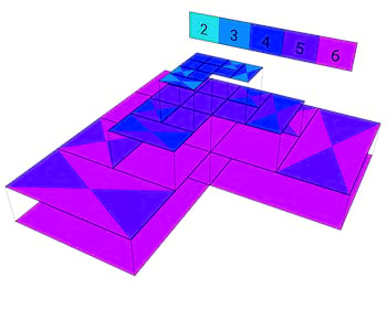
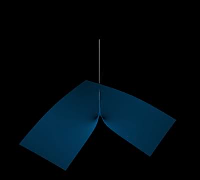
解图绘制
下面的解决方案图可以通过将解决方案导出为.vtk文件,并使用兼容的工具(如Visit)进行绘图来生成。

社区指南/行为准则
欢迎贡献、提问和错误报告!任何拉取请求、问题等都必须遵守Rust的行为准则。
有关如何为此项目做出贡献的更多详细信息,请参阅此处。
问题和错误报告应提交到问题标签页。
依赖项
~4.5MB
~90K SLoC