rust-bn

Rust 中的一个简单朴素贝叶斯模型。

基本思想来自 blayze，但 rust-bn 是一个 Rust 实现，并使用非常简单的 Rust HashMap<String, f64> 来在内存中保存模型。

稍后，应该很容易通过使用硬盘上的键值存储来增强它，以使模型持久化。

如何使用

简单地在本地检出此仓库并运行一些示例

git clone [email protected]:liufuyang/rust-nb.git

cargo run --example spam

# or run a more complex example, use --release to speed up train/test process
cargo run --example 20newsgroup_stopwords --release

然后您可以在 examples 文件夹中修改这些示例，并可能从那里构建自己的模型。

或者您可以在 Cargo.toml 中设置以在您的应用程序中使用此包

[dependencies]
...
rust_nb = "0.1.0"

只需创建一个如下所示的主函数。看看在训练和预测时一个简单的电子邮件垃圾邮件模型可能是什么样子。

extern crate rust_nb;

use rust_nb::{Feature, FeatureType, Model};

fn main() {
    let mut model = Model::new();

    let input_train = vec![
        (
            "spam".to_owned(),
            vec![
                Feature {
                    feature_type: FeatureType::Text,
                    name: "email.body".to_owned(),
                    value: "Good day dear beneficiary. This is Secretary to president of Benin republic is writing this email ... heritage, tax, dollars, money, credit card...".to_owned(),
                },
                Feature {
                    feature_type: FeatureType::Category,
                    name: "email.domain".to_owned(),
                    value: "evil.com".to_owned(),
                },
                Feature {
                    feature_type: FeatureType::Gaussian,
                    name: "email.n_words".to_owned(),
                    value: "482".to_owned(),
                },
            ],
        ),
        (
            "not spam".to_owned(),
            vec![
                Feature {
                    feature_type: FeatureType::Text,
                    name: "email.body".to_owned(),
                    value: "Hey bro, how's work these days, wanna join me for hotpot next week?".to_owned(),
                },
                Feature {
                    feature_type: FeatureType::Category,
                    name: "email.domain".to_owned(),
                    value: "gmail.com".to_owned(),
                },
                Feature {
                    feature_type: FeatureType::Gaussian,
                    name: "email.n_words".to_owned(),
                    value: "42".to_owned(),
                },
            ],
        ),
    ];

    model.train("Spam checker", &input_train);

    // test example 1
    let result = model.predict(
        "Spam checker",
        &vec![
            Feature {
                feature_type: FeatureType::Text,
                name: "email.body".to_owned(),
                value: "Hey bro, This is Secretary to president want to give you some money. Please give me your credit card number ..."
                    .to_owned(),
            },
            Feature {
                feature_type: FeatureType::Category,
                name: "email.domain".to_owned(),
                value: "example.com".to_owned(),
            },
            Feature {
                feature_type: FeatureType::Gaussian,
                name: "email.n_words".to_owned(),
                value: "288".to_owned(),
            },
        ],
    );

    println!("{:?}\n", result);
    assert!(result.get("spam").unwrap().abs() > 0.9);
    // result will be:
    // {"not spam": 0.04228956359881729, "spam": 0.9577104364011828}

    // test example 2
    let result = model.predict(
        "Spam checker",
        &vec![
            Feature {
                feature_type: FeatureType::Text,
                name: "email.body".to_owned(),
                value: "Hey bro, hotpot again?".to_owned(),
            },
            Feature {
                feature_type: FeatureType::Category,
                name: "email.domain".to_owned(),
                value: "gmail.com".to_owned(),
            },
            Feature {
                feature_type: FeatureType::Gaussian,
                name: "email.n_words".to_owned(),
                value: "10".to_owned(),
            },
        ],
    );

    println!("{:?}\n", result);
    assert!(result.get("not spam").unwrap().abs() > 0.9);
    // result will be:
    // {"spam": 0.03786816269284711, "not spam": 0.9621318373071529}
}

关于朴素贝叶斯模型（以及如何理解代码）

首先，让我们看一下只有两个类别和一个特征时的贝叶斯公式

正如我们所见，基于输入 x 的类别 1 和 2 的概率的分子是相同的（它们之和等于 1）。

因此，我们可以简单地只关注计算每个类别的分子部分，然后在最后将它们全部归一化，以得到每个类别的预测概率。

这也适用于类别数大于 2 的情况。

注意，这里我们使用 <= 符号表示我们可以在之后根据右边的值推断 p(c_n | x)，在我们完成了所有类别的计算后，其中类别的索引为 `n。

现在将这个扩展到我们拥有多个特征的情况，特征索引用 i 表示，让 X = x_1, x_2, ... x_i，我们得到

按照“朴素”的方式思考，每个特征的出现 x_i 是独立的，因此我们可以有

特征类型：多项式和分类

目前我们支持两种特征类型

• 分类特征：上述方程中的每个 x_i 都有不同的值
• 多项式（也称为文本特征）：上述方程中的每个 x_i 可以相同。例如，在计算单词数量以预测文档类的情况下，单词 apple 作为 x_i 可以出现多次，我们将其表示为 t_i（在代码中称为 inputFeatureCounts。）

也可以将 Categorical 特征视为 Multinomial 特征，但所有 t_i 的值都是 1。

因此，我们现在只关注 Multinomial 的方程。假设现在我们的 x_i 是唯一的单词，方程变为

存在许多小于 1 的值的乘法。为了防止数字太小而无法在计算机中以双精度表示，我们可以对每一边计算对数值

或

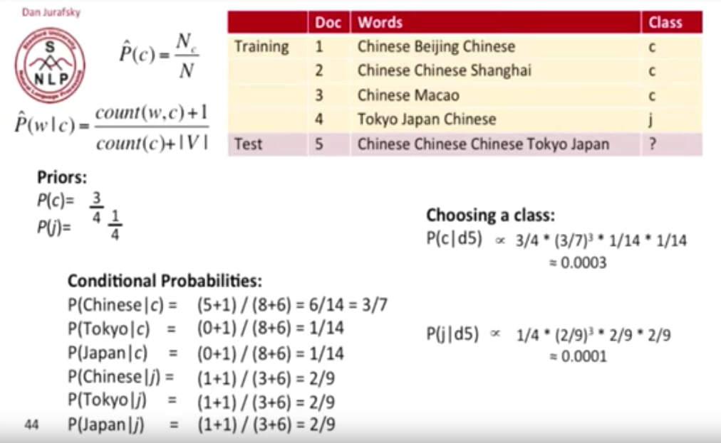
为了计算先验概率 p(c_n) 和条件概率 p(x_i| c_n)